Effect of time-dependent infectiousness on epidemic dynamics

Published

December 22, 2021

I’m very excited to share that a sole-authored work, “Effect of time-dependent infectiousness on epidemic dynamics”, is now out in Physical Review E! This started as a class project with Ren Stengel in Dan Larremore’s class, “Network Analysis and Modeling.” Over time, this morphed into the work that is currently published.

The central question that I answered was “How does adding a variable infection rate affect epidemics?” It turns out that many people have thought about this as well, and I read literature published 20 (!) years ago exploring this fact. I modified the SIR to include n infectious stages (traditionally called the SI^kR model), each stage corresponding to the infection rate at a point in time. It is called the viral load (VL) model for its ability to capture time-dependent transmissibility due to viral load.

I was able to use a combination of mean-field techniques and the “next-generation matrix” by Diekmann et al. to derive analytical expressions for the reproductive number. I derived this for both static and temporal networks with an arbitrary distribution of infectious rate functions.

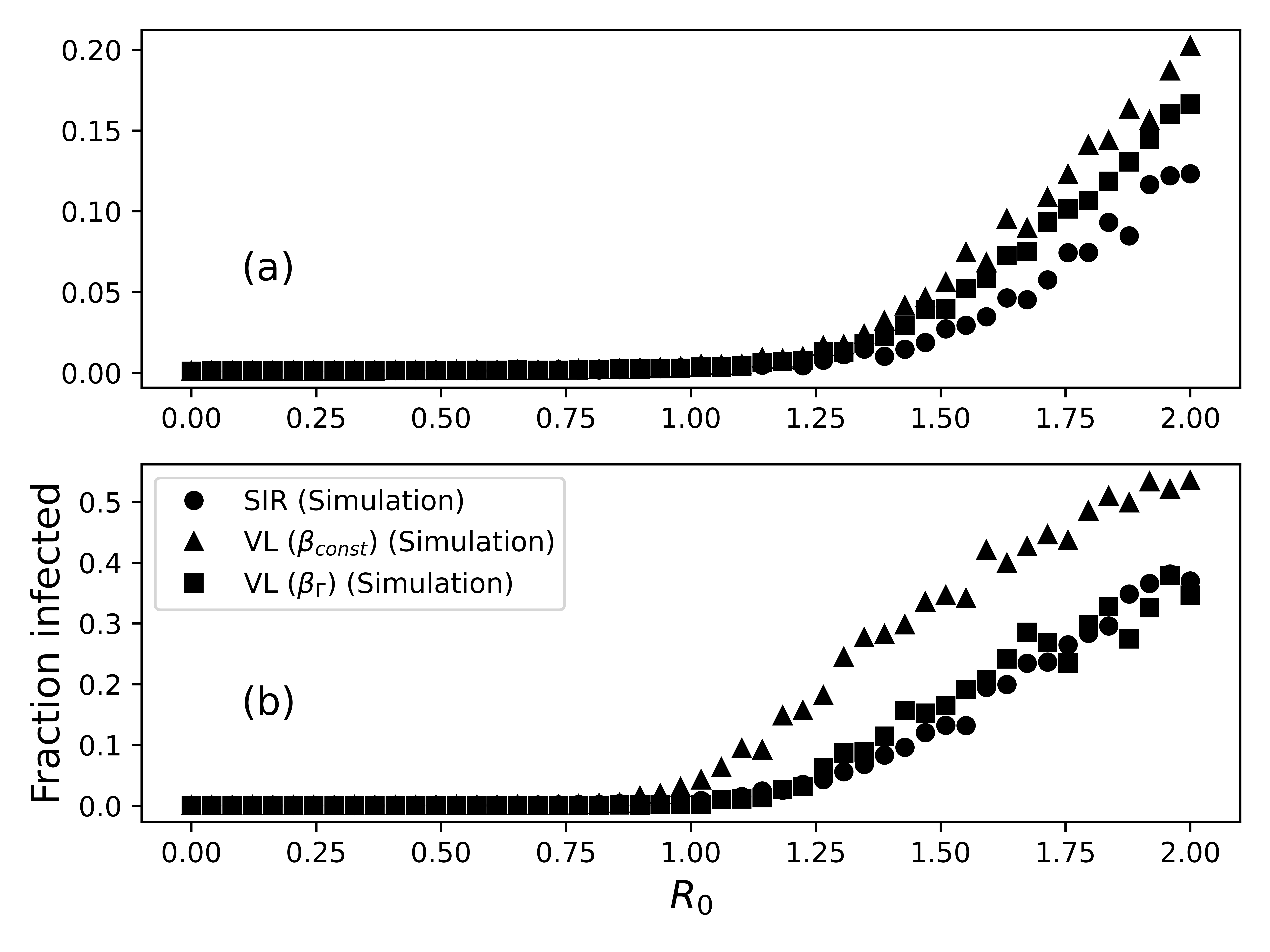
The reproductive number is exactly as you would expect from the SIR model when you let the infection rate equal the average of the infectious rate function. Here’s a plot of the epidemic extent with respect to the derived reproductive number.

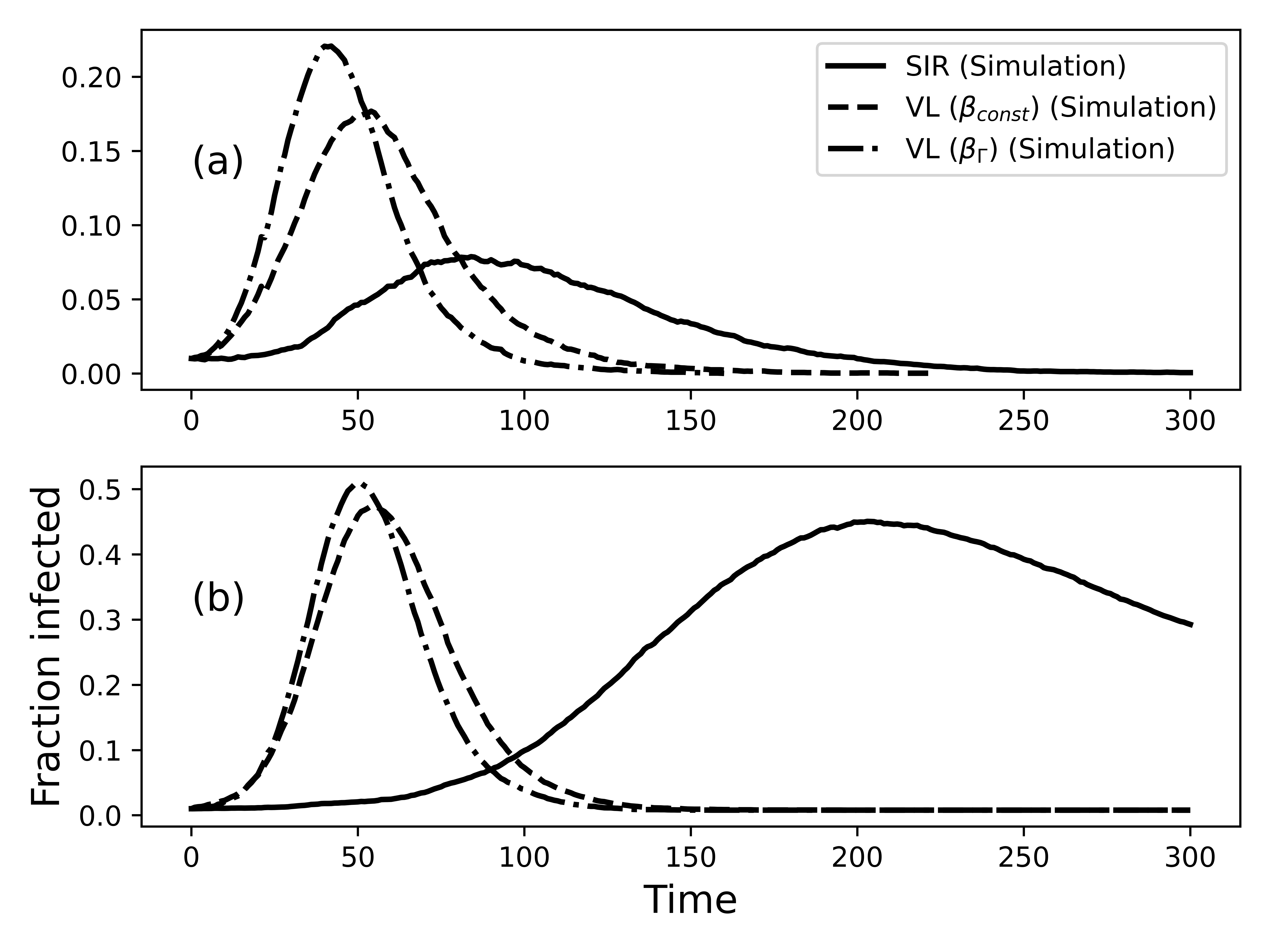
The VL model, however, strongly affects the time dynamics of how an epidemic unfolds; the time scale of the VL model is much shorter than the SIR model.

The epidemic trajectories of different contagion models

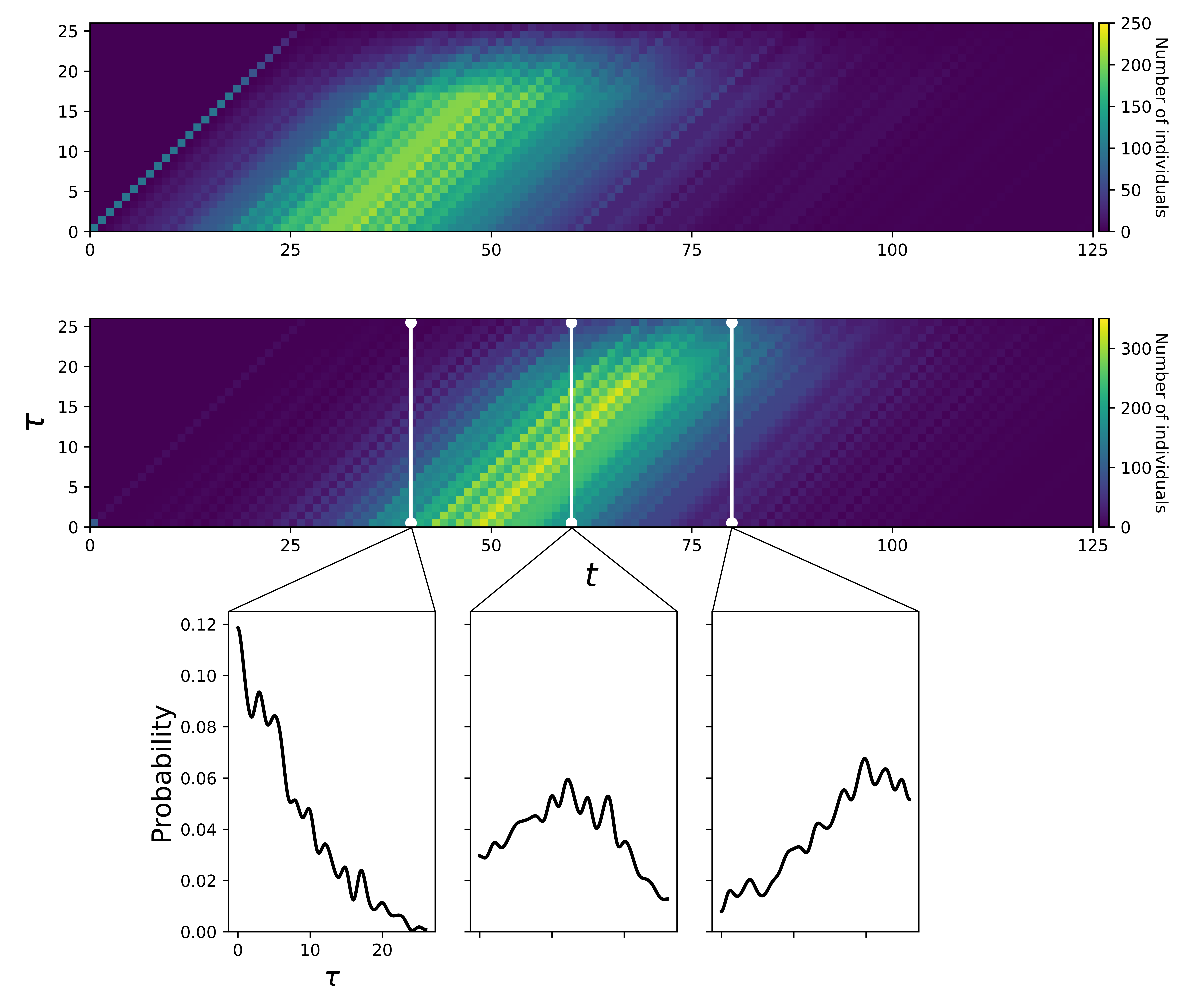
In addition, the infection propagates as a traveling wave of infection, which we demonstrate with numerical simulations and writing the VL model as a transport equation PDE with infectious boundary conditions.

The number of individuals infected for duration τ at time t for the configuration model (top) and the activity model (middle). The line plots (bottom) denote the probability distribution of τ at times 40, 60, and 80, which correspond to normalized vertical cross sections of I(t, \tau).

This project was especially significant for me as a researcher, because this paper helped me develop my voice. I am grateful to the reviewers for helping me strengthen the idea. A big shoutout to Ren Stengel, Dan Larremore, Juan G. Restrepo, and Subekshya Bidari for their help and input!